
Automatic Shape Matching (research project)
Introduction
The primary aim of this research project is to explore how complex shapes can be deconstructed into simpler, fundamental building blocks. In particular, the shape components examined here (though the curve segmentation algorithm is somewhat more fine-grained) are:
- Straight lines
- Maximal strictly convex segments (each exhibiting a single maximum curvature)
- Maximal strictly concave segments (each exhibiting a single minimum curvature)
Each component is characterized by various parameters, for example, the direction in which a concave segment opens. This “language” of shape provides a structured foundation for shape comparison. To match two shapes, the algorithm identifies corresponding components in the target shape by evaluating the similarity of their relative positions and component parameters. This process forms the core of this project.
There is a substantial body of literature on shape analysis and object detection that demonstrates diverse ways of exploiting contours. For example, see [1], [2], [4], [8], or [9]. However, to the best of my knowledge, no existing research employs the specific shape components and matching algorithm developed in this project.
Our approach integrates shape decomposition with object segmentation models, specifically the Segment Anything Model (SAM) [3] by Meta AI. First, SAM is used to extract object contours. Then, using my shape decomposition algorithm and a matching procedure, the shape components of a template are matched to the corresponding components of another shape.
Before delving into technical details, here are some visual examples of the final results.
Results
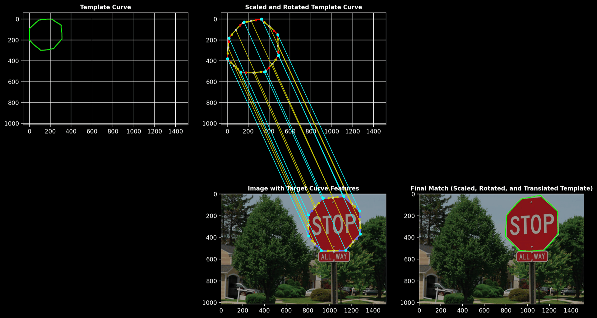
Stop Sign
- Template curve: hand-drawn
- Target curve: contour of a mask obtained using SAM
Process Overview:
The images below illustrate how the stop sign is broken down into its basic components and how these components are matched between the template and the segmented image.
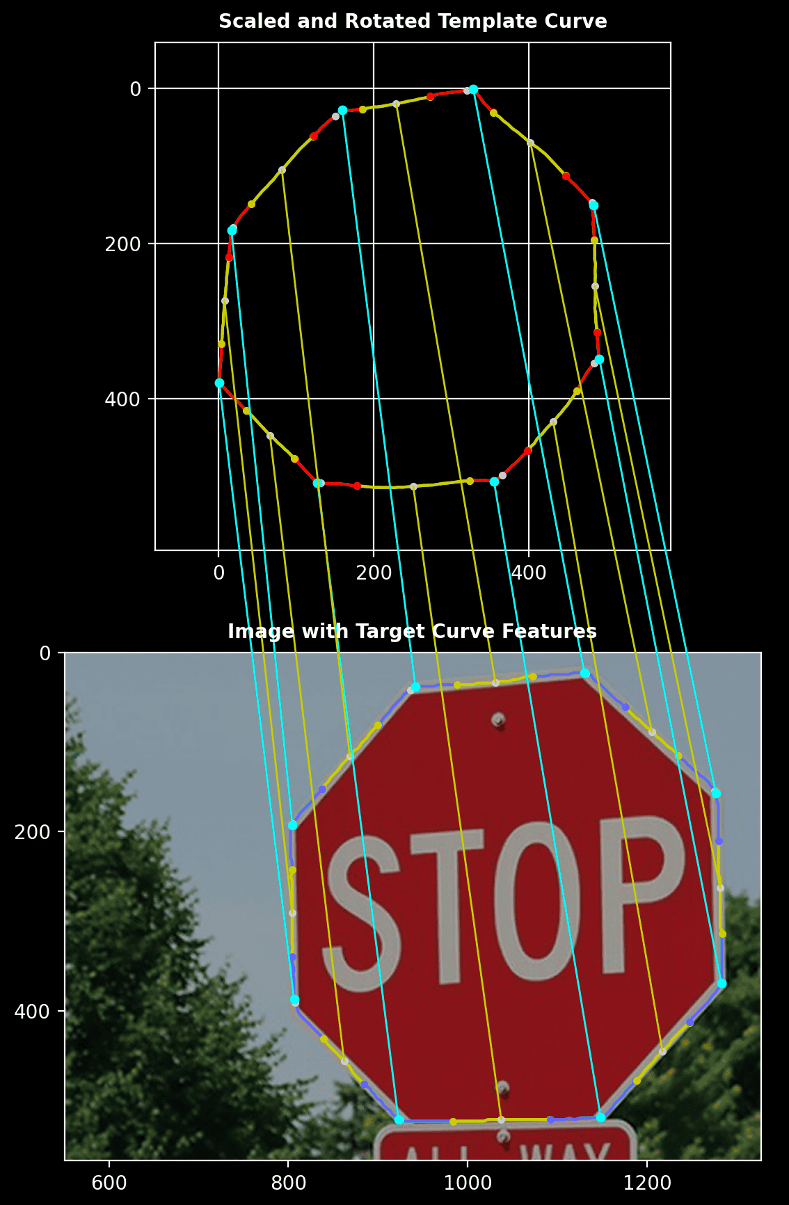
Zoomed-In View:
A closer view shows the alignment of specific segments between the hand-drawn template and the extracted contour.
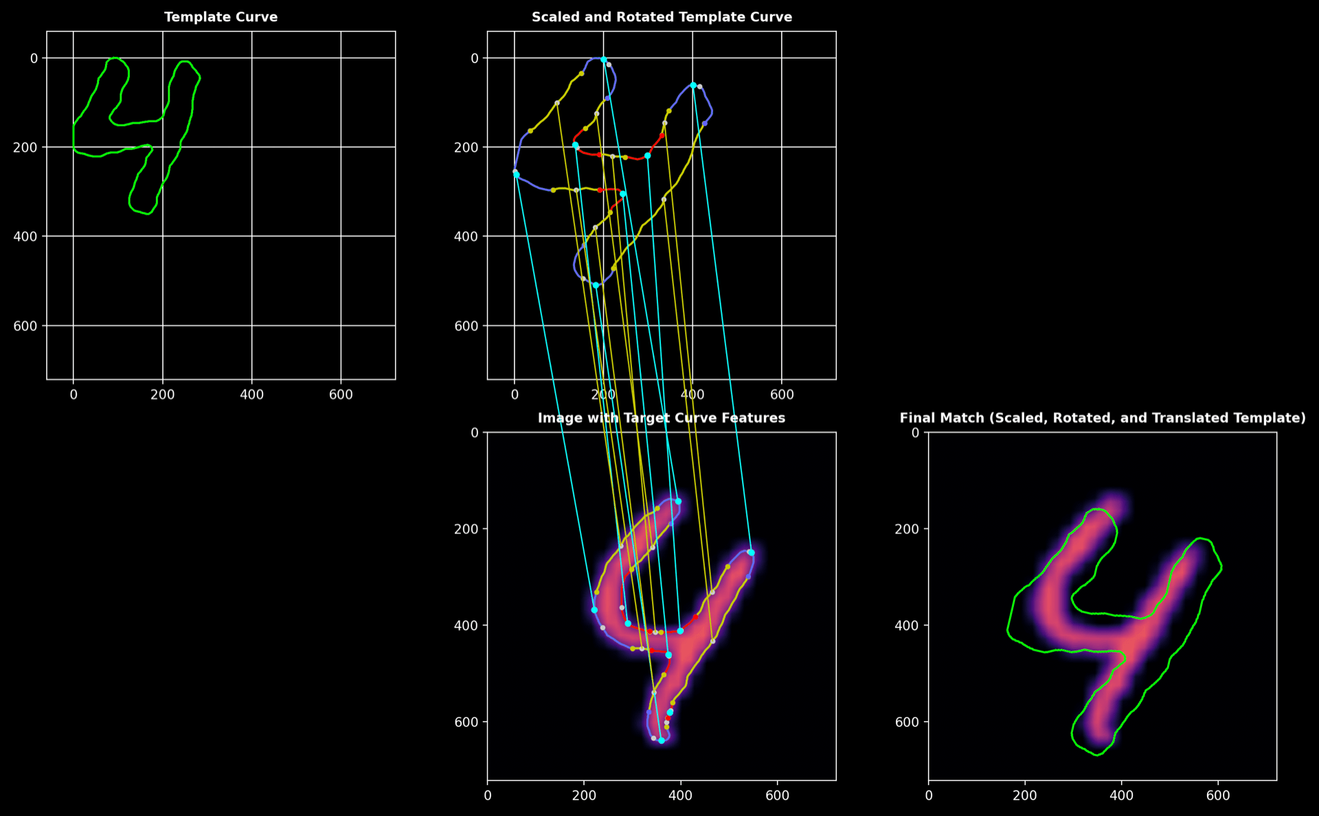
MNIST Digit Matching
- Template curve: contour of a “4” from the MNIST dataset
- Target curve: contour of another “4” from the MNIST dataset
Process Overview:
Below, you can see the deconstruction of the MNIST digit “4,” highlighting the correspondence between the template and the segmented contour.
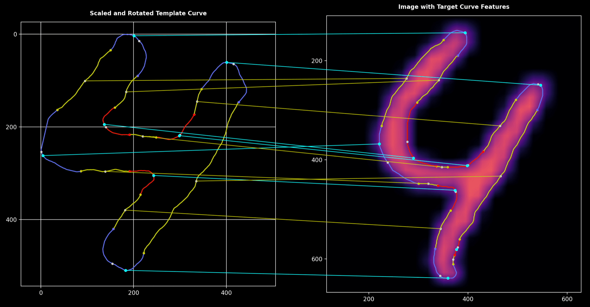
Zoomed-In View:
The zoomed view reveals the precise matching of segments and how the algorithm handles subtle differences.
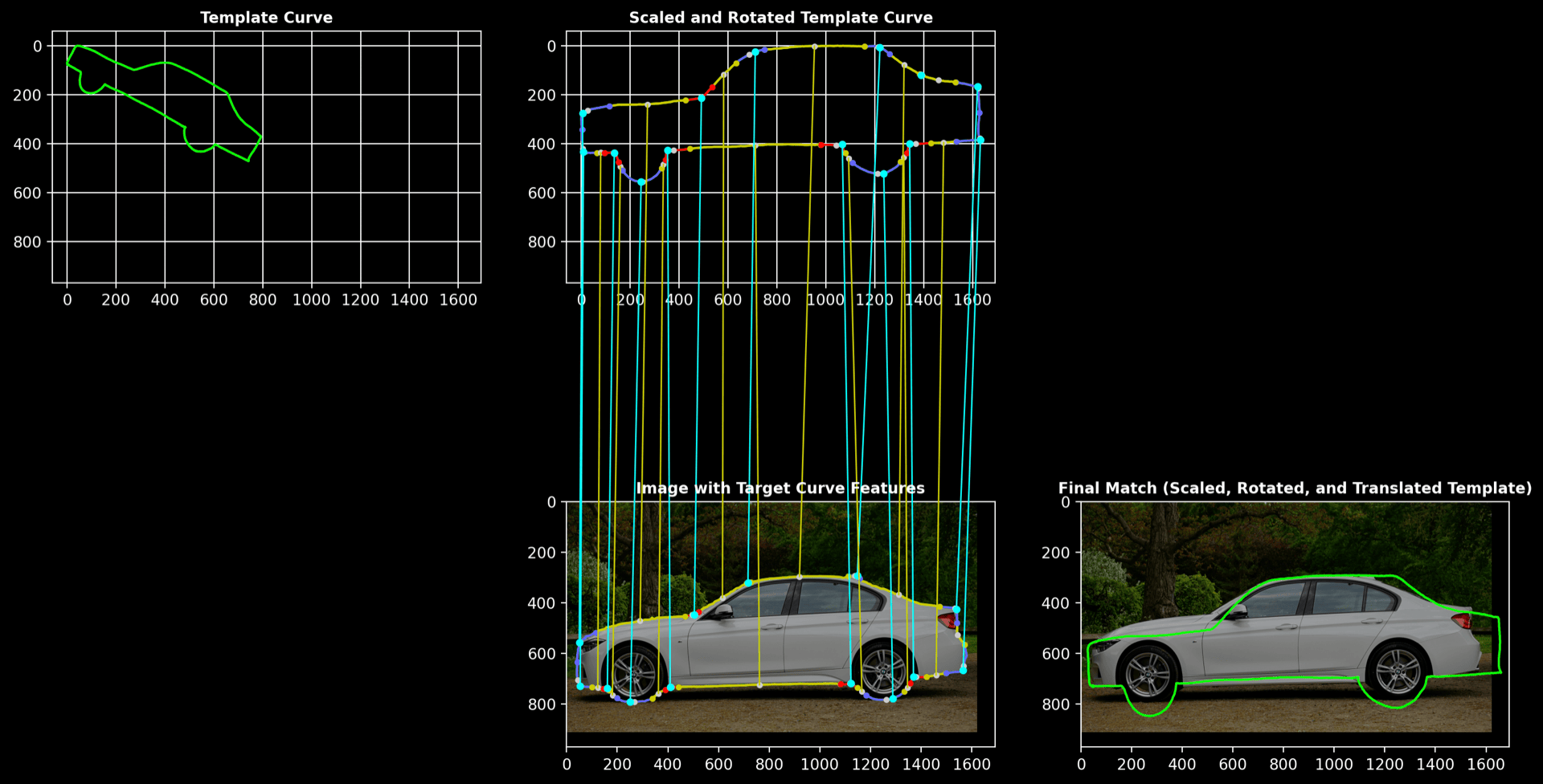
Car
- Template curve: hand-drawn car shape
- Target curve: contour of a car obtained using SAM
Process Overview:
The visualization below shows how a complex car outline is simplified into core components and then matched between the template and the segmented shape.
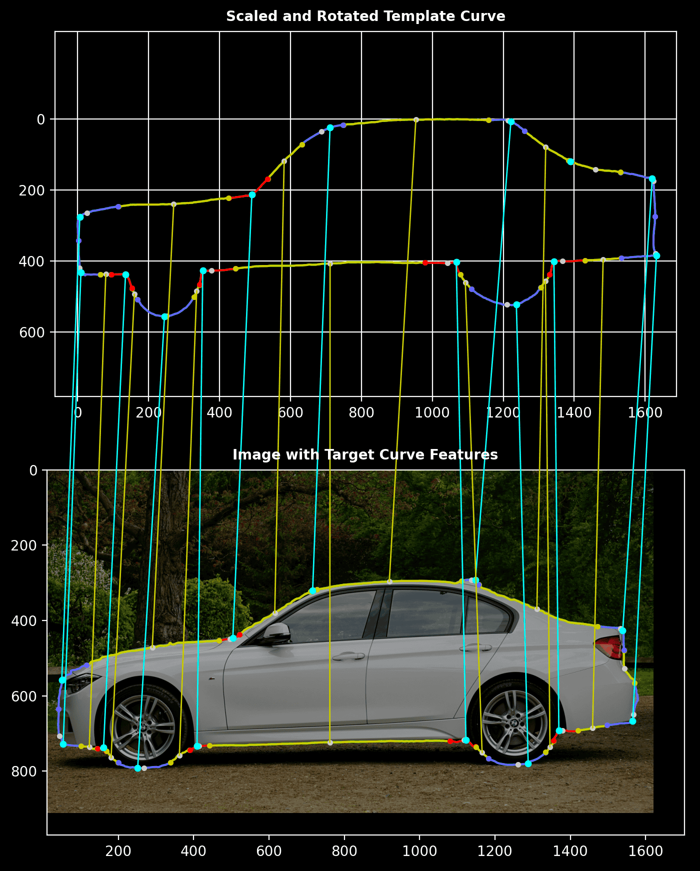
Zoomed-In View:
This closer look highlights the correspondence between segments of the hand-drawn car and the segmented shape.
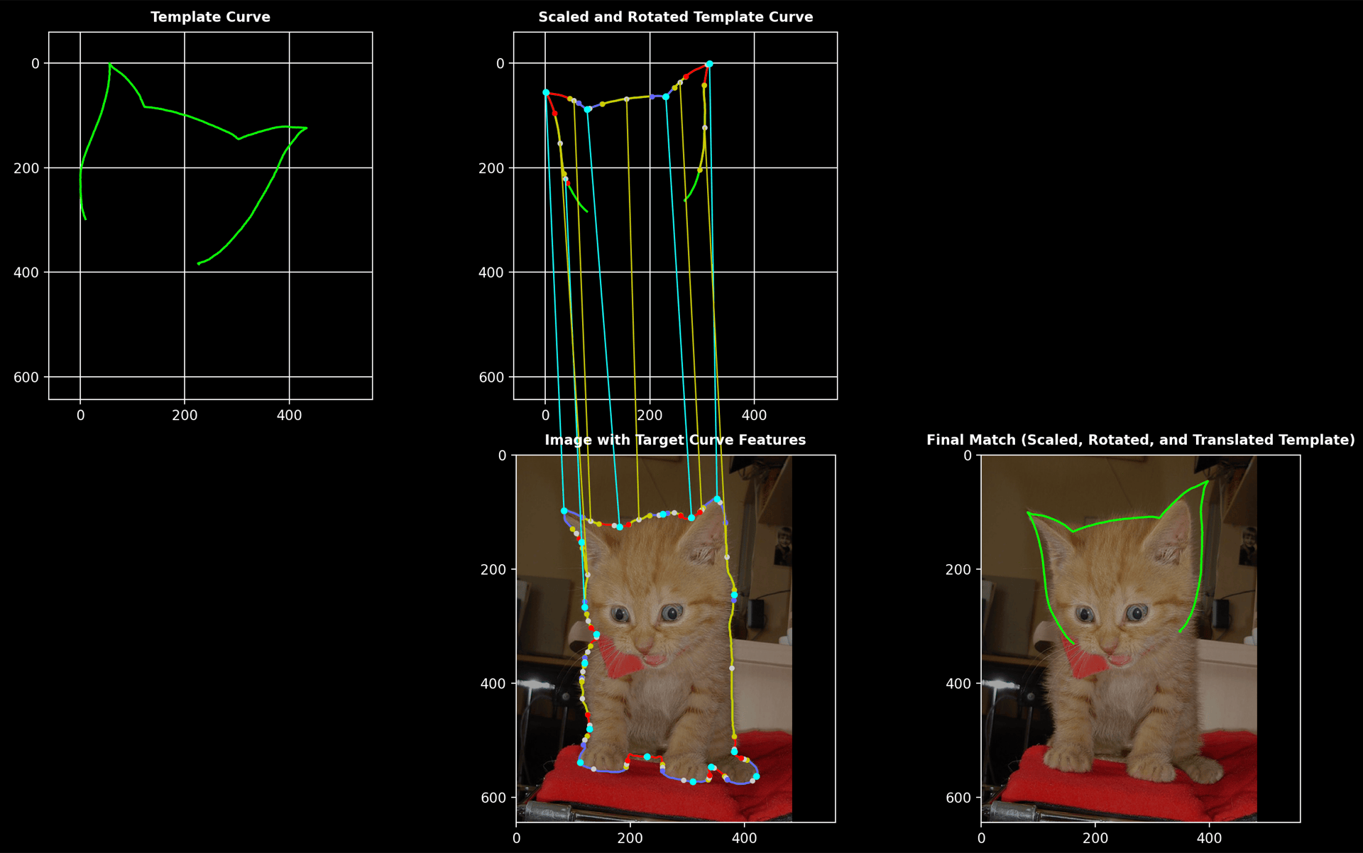
Cat
- Template curve: hand-drawn cat shape
- Target curve: contour of a cat obtained using SAM
Process Overview:
Here, the transformation of a cat sketch into fundamental shapes is presented, along with the matching that aligns the hand-drawn and segmented contours.
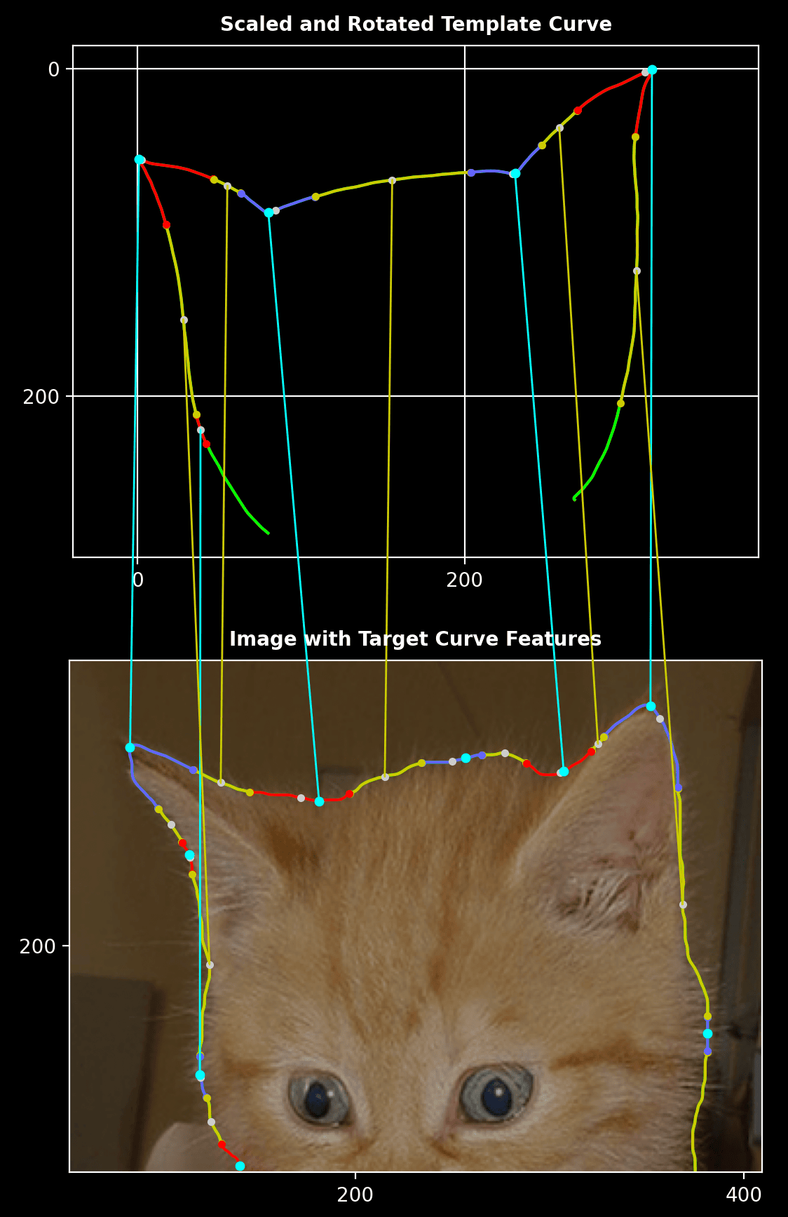
Zoomed-In View:
A magnified view focuses on the alignment of specific features and contours in the cat shape.
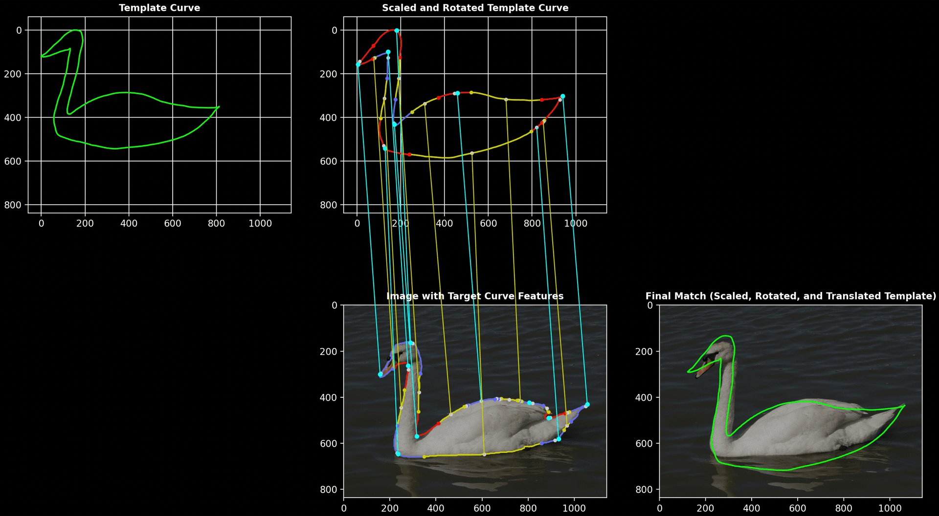
Swan
- Template curve: hand-drawn swan shape
- Target curve: contour of a swan obtained using SAM
Process Overview:
The sequence below shows the deconstruction of a swan outline into basic shapes, as well as the subsequent matching between the template and segmented shapes.
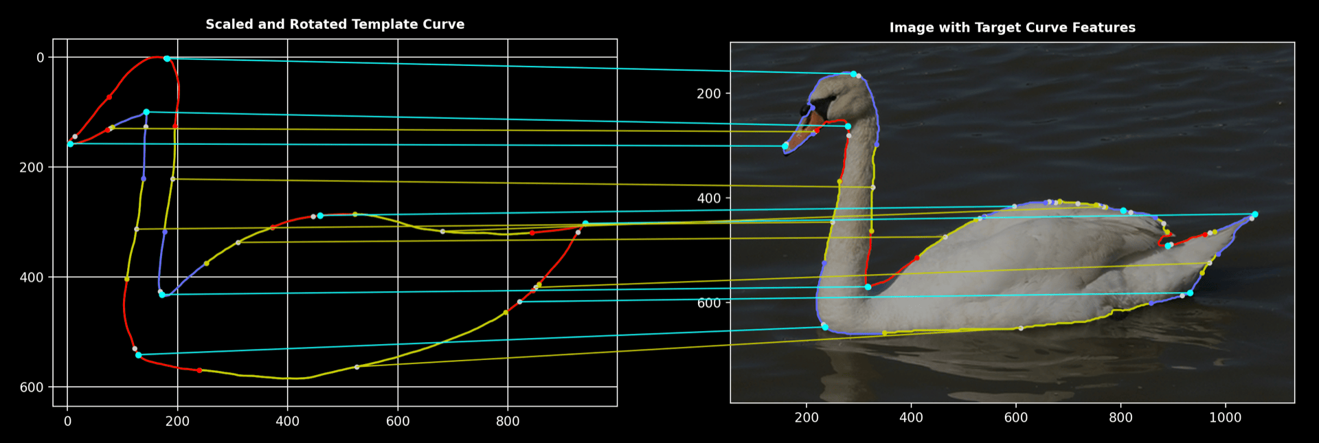
Zoomed-In View:
A detailed close-up illustrates how precisely the features of the swan’s shape are matched.
Some Technical Details
Measuring Curvature of Discrete Plane Curves
Curvature of a Plane Curve
Let \(\boldsymbol{\gamma}(s) = (x(s),\,y(s))\) be a twice-differentiable plane curve parameterized by arc length \(s\), such that \(\|\boldsymbol{\gamma}'(s)\| = 1\). The curvature \(\kappa(s)\) at a point \(s\) is defined as the magnitude of the second derivative of \(\boldsymbol{\gamma}\) with respect to \(s\):
\[\kappa(s) = \|\boldsymbol{\gamma}''(s)\|.\]Equivalently, \(\kappa(s)\) measures how quickly the unit tangent vector rotates as \(s\) increases. High curvature corresponds to a sharper bend, while zero curvature indicates a perfectly straight segment.
Discrete Curves and Curvature Measurement
In many practical settings (e.g., image analysis), curves are represented discretely as a sequence of points. To adapt the continuous definition of curvature to such discrete curves, the following preprocessing steps are employed:
-
Initial Arc-Length Parameterization
Resample the curve so that consecutive points are equally spaced by a fixed Euclidean distance, approximating a continuous arc-length parameterization. -
Smoothing the Curve
After the initial parameterization, smooth the curve (e.g., by applying a Gaussian filter) to reduce noise. For closed curves, perform smoothing in a wraparound manner to preserve continuity at the endpoints. -
Second Arc-Length Parameterization
Since smoothing alters the spacing between points, resample the curve a second time to ensure uniform spacing.
I developed this procedure independently, but later discovered that it aligns with the approach in [6], where both \(x(s)\) and \(y(s)\) are convolved with a Gaussian kernel. In addition, [7] offers an overview of the material presented in [6], while [5] addresses the problem of curve shrinkage that occurs during Gaussian smoothing.
Curvature Definition Using Bar Length
To estimate the signed curvature at each point \(p\) of the discrete, arc-length-parameterized curve, we pick a fixed bar length parameter \(L\) (for instance, \(L = 2\)). The process is:
- Select Neighboring Points
- From point \(p\), move a distance \(L\) backwards along the curve to find point \(a\).
- Move a distance \(L\) forwards along the curve to find point \(b\).
- Compute the Signed Curvature Angle
- Determine the angle \(\theta\) between vectors \(\overrightarrow{pa}\) and \(\overrightarrow{pb}\).
- Assign a sign to \(\theta\) based on the orientation:
- Positive if moving from \(\mathbf{a}\) to \(\mathbf{p}\) to \(\mathbf{b}\) is a counterclockwise turn.
- Negative if it is a clockwise turn.
Thus, the signed curvature at \(p\) is: \(\kappa(p) = \pm \,\angle\big(\overrightarrow{pa}, \,\overrightarrow{pb}\big).\)
The bar length \(L\) acts as a scale parameter:
- Larger \(L\): smooths out minor fluctuations, giving a broader notion of curvature.
- Smaller \(L\): more sensitive to local bends, capturing finer detail.
In practice, \(\kappa(p)\) is thresholded; if \(\kappa(p)\) is below some small threshold, it is set to \(0\).
Shape Component Definition
For shape matching, we focus on the following key components. This overview is slightly simplified; the underlying shape component extractor can handle additional refinements.
-
Straight Line
A maximal subsegment where the curvature \(\kappa(p) = 0\) (after applying a threshold). In shape matching, the midpoint and angle of each line serve as key attributes. - Maximal Strictly Convex Curve with a Single Peak (Convex Subcurve)
A subsegment with \(\kappa(p) > 0\) (strict convexity) containing a single local maximum. In shape matching, we utilize its facing angle and the degree to which the curve is “open” (see Fig. 1):- Start Angle and End Angle: Approximations of the tangent orientations at the subcurve’s start and end points.
- Facing Angle: The average of the start and end angles.
- Turning Angle: The absolute difference between the start and end angles.
- Maximal Strictly Concave Curve with a Single Peak (Concave Subcurve)
Defined similarly to a convex subcurve, but with \(\kappa(p) < 0\).
The convexity or concavity of a subcurve depends on the direction in which the curve is traversed. In the results section above, red segments represent convex subcurves, while blue segments represent concave subcurves.
Comparing Shapes
Let \(C_1\) denote the template curve and \(C_2\) denote the target curve. The goal of shape comparison is to determine the optimal parameters that best align \(C_1\) with \(C_2\). These parameters include:
- The bar length to use for \(C_1\) to extract its subcurves and straight-line features.
- The bar length to use for \(C_2\) to extract its subcurves and straight-line features.
- The scaling factor to apply to \(C_1\).
- The rotation angle to apply to \(C_1\).
- The translation vector to apply to \(C_1\).
The algorithm exhaustively explores various combinations of these parameters. For each configuration, it extracts the corresponding shape components from both \(C_1\) and \(C_2\), computes the matches, and assigns a similarity score, finally selecting the configuration with the highest overall score.
Translation Matching:
Once the scaling, rotation, and bar length parameters are fixed, the algorithm extracts the features from both curves. Suppose \(C_1\) yields subcurves \(a_1, a_2, \ldots, a_k\) and \(C_2\) yields subcurves \(b_1, b_2, \ldots, b_l\) (and similarly for the straight-line segments). The algorithm considers all possible pairings; for example, mapping \(a_1\) to \(b_1\) yields a candidate translation vector \(t\). Then, \(C_1\) is translated by \(t\), and for each feature in \(C_1\) the nearest corresponding feature in \(C_2\) is identified based solely on relative position. Once these correspondences are established, a similarity score is computed for that configuration.
Similarity Computation
The similarity between \(C_1\) and \(C_2\) is computed by evaluating the geometric and angular differences between each pair of matched features. A higher value (close to 1) indicates more similar, and a lower value (close to 0) less similar. For a given pair of matched features, the similarity score is calculated using Gaussian-like functions. For convex (or concave) subcurves, the score is computed as:
\[S = \left( \exp\left(-\frac{(\Delta \alpha)^2}{2\sigma_{\alpha}^2}\right) \times \exp\left(-\frac{(\Delta \theta)^2}{2\sigma_{\theta}^2}\right) \times \exp\left(-\frac{d^2}{2\sigma_d^2}\right) \right) - \epsilon_1,\]where:
- \(\Delta \alpha\) is the difference in facing angles,
- \(\Delta \theta\) is the difference in total turning angles,
- \(d\) is the Euclidean distance between the corresponding feature points,
- \(\sigma_{\alpha}\), \(\sigma_{\theta}\), and \(\sigma_d\) are the respective width parameters,
- and \(\epsilon\) is a small constant.
Note: The product of the Gaussian functions is always non-negative. Subtracting \(\epsilon_1\) ensures that if the computed similarity for a feature is below \(\epsilon_1\), then the similarity score is negative. Such a score is deemed to low, and that subcurve match is removed.
For straight-line features, the similarity is computed as:
\[S = \left( \exp\left(-\frac{(\Delta \phi)^2}{2\sigma_{\phi}^2}\right) \times \exp\left(-\frac{d^2}{2\sigma_d^2}\right) \right) - \epsilon_2,\]where \(\Delta \phi\) is the difference in line orientations and \(\sigma_{\phi}\) is its corresponding width parameter.
Note: The role \(\epsilon_2\) is the same as the role of \(\epsilon_1\) above.
The overall similarity score for a particular alignment is obtained by summing these scores over all matched features and normalizing by the total number of features. This comprehensive measure captures both positional and angular discrepancies between the two curves.
Optimal Matching
The complete matching procedure is executed over all possible combinations of transformations (scaling, rotation, and bar lengths) and translations. The configuration that yields the highest overall similarity score is selected as the optimal match. This final alignment specifies:
- The exact scale, rotation, and bar lengths used for segmenting \(C_1\) and \(C_2\).
- The translation vector that best aligns \(C_1\) with \(C_2\).
- The corresponding pairings of straight lines, convex subcurves, and concave subcurves between the two shapes.
This comprehensive process ensures that even when \(C_1\) and \(C_2\) differ in size, orientation, or smoothness, their intrinsic geometric components are reasonably well-matched.
Opportunities for Improvements
While the current algorithm provides a robust framework for matching shapes, several enhancements could further improve its efficiency and accuracy:
-
Faster Parameter Optimization:
The matching algorithm currently explores all possible parameter settings exhaustively. Incorporating Bayesian Optimization using Gaussian Processes could dramatically reduce computation time by intelligently guiding the search for optimal parameters. -
Enhanced Feature Matching:
At present, the algorithm first matches straight lines and subcurves based solely on location, and then computes similarity scores between these matched pairs. A more integrated approach, where the similarity score is considered during the matching process, could improve the overall robustness and accuracy of the feature pairing. -
Learning Comparison Parameters:
The various width parameters (e.g., \(\sigma_{\alpha}\), \(\sigma_{\theta}\), \(\sigma_d\), etc.) are currently set heuristically. These parameters could be optimized or even learned using supervised learning techniques on a labeled dataset, ensuring that the similarity measures are better tuned to the specific characteristics of the shapes being compared. -
Multi-Curve Matching:
The present implementation handles the matching of a single pair of curves (C1 and C2). Future enhancements could extend the algorithm to compare entire sets of curves, enabling applications such as shape clustering or multi-object recognition.
Some References
-
Belongie, S., Malik, J., & Puzicha, S. (2002).
Shape matching and object recognition using shape contexts.
IEEE Transactions on Pattern Analysis and Machine Intelligence, 24(4), 509-522.
DOI: 10.1109/34.993558 -
Blum, H. (1967).
A transformation for extracting new descriptors of shape.
In W. Weiant Wathen-Dunn (Ed.), Models for the Perception of Speech and Visual Form (pp. 362–380). MIT Press, Cambridge.
http://pageperso.lif.univ-mrs.fr/~edouard.thiel/rech/1967-blum.pdf -
Kirillov, A., Mintun, E., Ravi, N., Mao, H., Rolland, C., Gustafson, L., Xiao, T., Whitehead, S., Berg, A. C., Lo, W.-Y., Dollár, P., & Girshick, R. (2023).
Segment Anything.
In 2023 IEEE/CVF International Conference on Computer Vision (ICCV), 3992-4003.
DOI: 10.1109/ICCV51070.2023.00371 -
Leavers, V. F. (1992).
Shape Detection in Computer Vision Using the Hough Transform.
Springer-Verlag London Limited, 1992.
DOI: 10.1007/978-1-4471-1940-1 -
Lowe, D. G. (1989).
Organization of smooth image curves at multiple scales.
International Journal of Computer Vision, 3, 119–130.
DOI: 10.1007/BF00126428 -
Mokhtarian, F., & Mackworth, A. (1986).
Scale-Based Description and Recognition of Planar Curves and Two-Dimensional Shapes.
IEEE Transactions on Pattern Analysis and Machine Intelligence, PAMI-8(1), 34-43.
DOI: 10.1109/TPAMI.1986.4767750 -
Mokhtarian, F., & Bober, M. (2003).
Curvature Scale Space Representation: Theory, Applications, and MPEG-7 Standardization.
Kluwer Academic Publishers / Springer.
DOI: 10.1007/978-94-017-0343-7 -
Schindler, K., & Suter, D. (2008).
Object detection by global contour shape.
Pattern Recognition, 41(12), 3736-3748.
DOI: 10.1016/j.patcog.2008.05.025 -
Šukilović, T. (2015).
Curvature based shape detection.
Computational Geometry, 48(3), 180-188.
DOI: 10.1016/j.comgeo.2014.09.005