Fisheye to Rectilinear: A Custom Dewarping Journey (project)
Introduction
In this project, I developed a tool to transform fisheye camera footage into a rectilinear (perspective-like) view. Although libraries like OpenCV can dewarp fisheye images, they do not provide fine-grained control over which portion of the fisheye view is converted. To fill that gap, I derived the geometry and math from scratch, enabling precise selection of the dewarping region. No existing “dewarping” library is used; every step of my fisheye projection model is coded by hand.
High-level project description
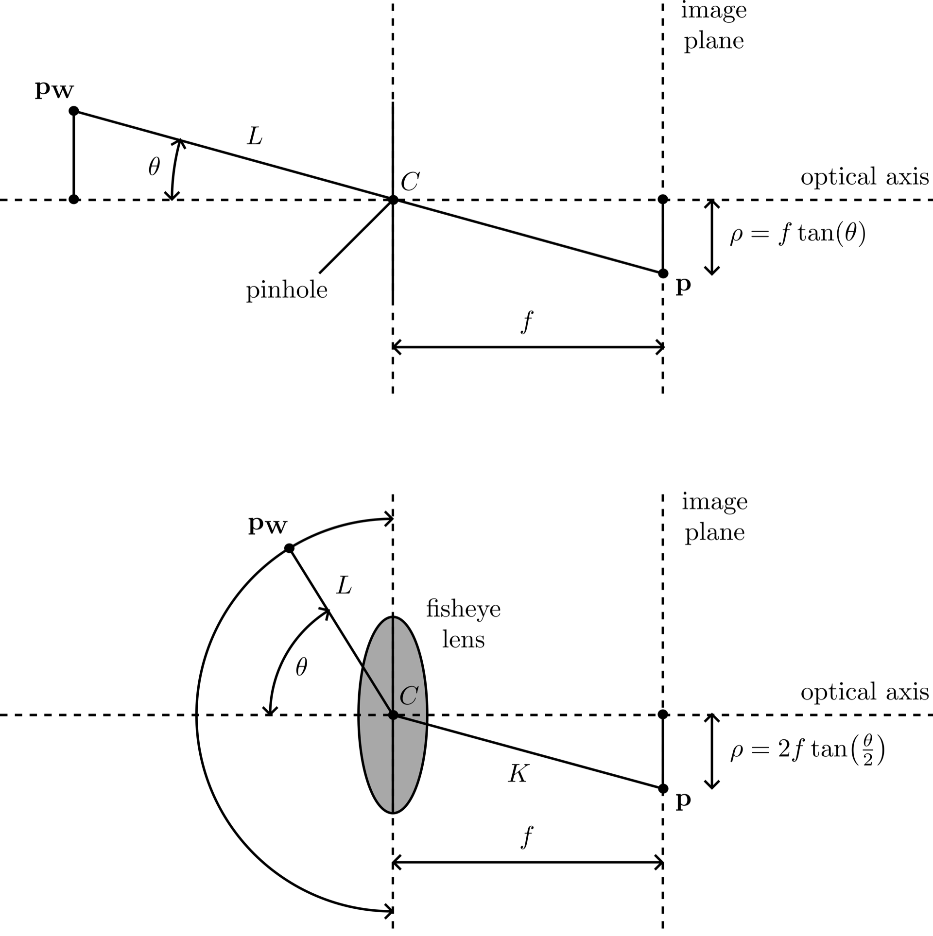
The fisheye camera model I use [1, 2] can be viewed as a generalization of the pinhole camera model. First, consider the pinhole model (Fig. 2, top). The camera coordinate frame is defined so that the pinhole (camera center) \(C\) is at the origin. In Fig. 2, the positive \(z\)-axis extends forward, the positive \(x\)-axis extends to the left, and the positive \(y\)-axis extends upward. The image plane lies behind the optical center.
Pinhole model
Given a point \(\mathbf{p_W}\) in the world, I draw a line segment \(L\) from \(\mathbf{p_W}\) to \(C\). For a pinhole camera, \(L\) is extended beyond \(C\) in the same direction until it intersects the image plane at \(\mathbf{p}\). The distance \(\rho\) between \(\mathbf{p}\) and the central (optical) axis is given by \(\rho = f \,\tan(\theta),\) where \(f\) is the focal length parameter, and \(\theta\) is the angle between segment \(L\) and the optical axis. Each lens type has its own projection formula, describing how the intersection with the image plane depends on the entrance angle [3].
Fisheye model
In the fisheye model (Fig. 2, bottom), the projection from \(C\) to the image plane differs from the pinhole approach. I still define a line segment \(L\) from \(\mathbf{p_W}\) to \(C\), but instead of extending \(L\) beyond \(C\) in the same direction, I introduce a new segment \(K\). Both \(L\) and \(K\) lie in the plane determined by \(L\) and the optical axis. Let \(\theta\) be the angle between \(L\) and the optical axis. The fisheye lens formula specifies how \(K\) is oriented, so that its endpoint on the image plane is at a distance
\[\rho = g(\theta)\]from the optical axis. Here, \(g(\theta)\) is the fisheye projection function. Examples include:
-
Equidistant
\(\rho = f\,\theta\) -
Stereographic
\(\rho = 2f \,\tan\bigl(\tfrac{\theta}{2}\bigr)\) -
Equisolid
\(\rho = 2f \,\sin\bigl(\tfrac{\theta}{2}\bigr)\) -
Orthographic
\(\rho = f \,\sin(\theta)\)
Here, \(f\) is a parameter that sets the lens scale, and \(\theta\) ranges from 0 (along the optical axis) up to the lens’s maximum field of view.
Dewarping process
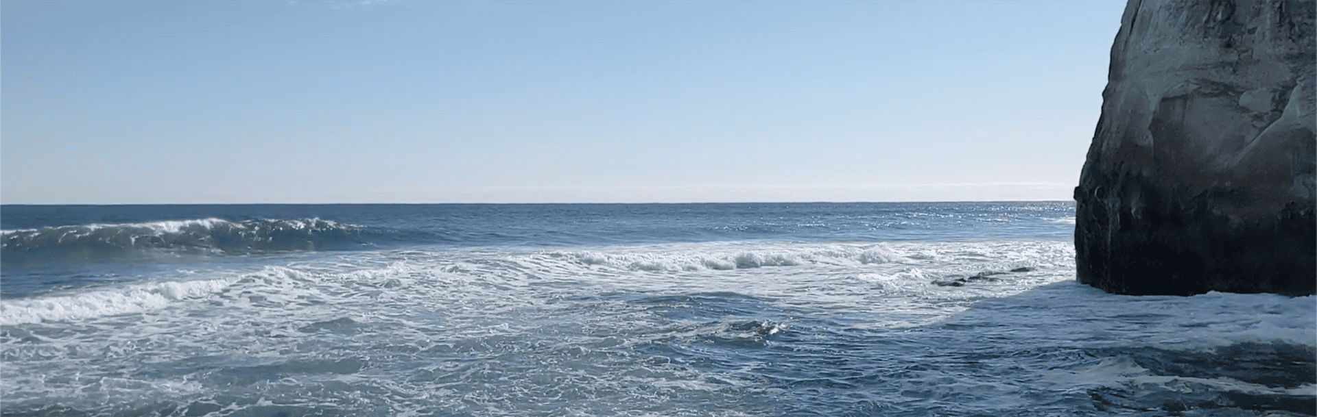
Once my fisheye projection model is defined, I invert it to produce a rectilinear image. The animation at the top of this page (Fig. 1) shows one example of this transformation. Conceptually, the process involves:
-
Select a virtual view plane
I place a rectangle \(R\) perpendicular to the \(z\)-axis, intersecting it at \(z = 1\). One edge is parallel to the \(x\)-axis, and the other to the \(y\)-axis. A grid \(G\) is then overlaid on this rectangle.My tool supports several adjustments for \(R\):
- Field of view (horizontal & vertical) in degrees
- Rotation around the \(x\)-, \(y\)-, and \(z\)-axes
- Grid density, which affects output resolution
-
Trace rays to determine colors
For each point \(\mathbf{v} \in G\), I use the fisheye model to find where \(\mathbf{v}\) maps onto the original fisheye image. First, I compute the angle \(\theta\) from the optical axis and then use the fisheye formula to get the corresponding distance (radius) \(\rho\) on the image plane. This information, along with the angular position around the optical axis, yields a location on the fisheye image that may not fall exactly on a pixel center. In such cases, surrounding pixels are sampled and linearly interpolated to estimate the correct color, ensuring a smooth result and reducing aliasing. I then assign this interpolated color value to \(\mathbf{v}\) in the output image.
By applying these steps to every point in \(G\), I form a rectilinear view of the scene on \(R\), effectively “unwrapping” the fisheye source.
References
1. Automatic calibration of fish-eye cameras from automotive video sequences
3. Bettonvil, F. (2005). “Imaging: Fisheye lenses,” WGN, the Journal of the IMO, 33(1), 9.
Code availability:
Not publicly available due to contractual obligations.
Video Attribution:
Fisheye footage by Videvo (CC-BY 3.0)